Geo-experimentation in smaller markets: why the US playbook fails (and how to fix it)

Most online guides, documentation, and open-source packages for marketing geo-lift experiments (such as Meta’s GeoLift, Google’s Trimmed Match, or CausalPy) share a quiet, underlying assumption: you are running your test across a massive, geographically spread-out market like the United States.

In the US, splitting the country into dozens of Designated Market Areas (DMAs) or states works reasonably well. Each region is geographically huge, self-contained, and economically distinct. But when you try applying those exact same frameworks to smaller European countries — like Belgium, Denmark, Austria, or Czechia — the standard playbook breaks down fast.

When designing and evaluating geo-experiments in compact markets, smaller geography introduces physical, structural, and behavioral challenges that automated statistical tools completely gloss over.

1. The statistical trap: tighter fits, dirtier data

When setting up a matching-based geo-experiment (like synthetic control or trimmed match), the optimization algorithm evaluates quality using pre-period fit — how closely a candidate pool of control regions mirrored your treatment regions before your campaign launched.

If you let an automated optimizer choose the best split, it will almost always prefer finer geographic partitions (e.g. postal codes or small administrative NUTS-3 districts). More candidate units mean more degrees of freedom, which produces tighter historical alignment curves on paper.

The core tradeoff: finer geographic partitions improve statistical pre-fit on paper, but they systematically worsen every real-world contamination vector in practice. Statistical models look backward at historical sales correlation. They have no physical awareness of whether an ad delivered to “District A” today will cause a consumer to commute and spend money in “District B” tomorrow. The statistics-side view of geographic partitioning is systematically optimistic.

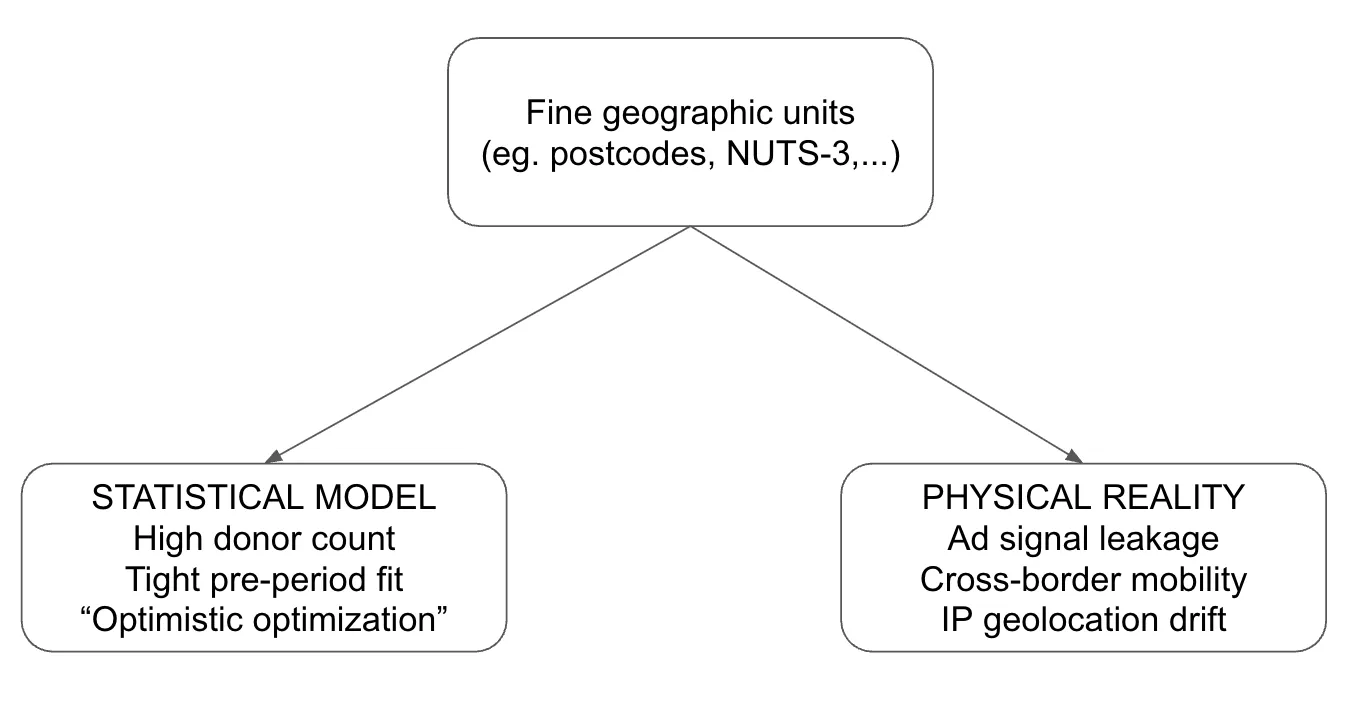
2. The three contamination vectors you must clear

To establish true causal incrementality in a compact market, you must clear three independent contamination vectors. Media selection addresses only the first; measurement keying addresses only the second; geographic unit size affects all three.

Vector 1: Delivery contamination (the ad signal crosses the border)

• The mechanism: Broad media broadcast boundaries rarely align with local administrative lines. Digital geotargeting (paid social, programmatic display, YouTube) relies on probabilistic edge signals (cellular towers, Wi-Fi location, VPNs) that bleed across borders.
• How to address it: Use media channels with strict, auditable geo-delivery: platforms with high-quality explicit geo-targeting (at the level you used for test design — different ad platforms use different geo-targeting), localized print with verified distribution logistics, or geo-fenced Out-of-Home (OOH). And always be aware of how the platform actually geo-targets (how it estimates the user’s location, or whether it uses “geo-intent” data instead).

Vector 2: Mobility contamination (people cross the border)

• The mechanism: In smaller countries, cross-region commuting and travel are daily norms. An individual living in Region A commutes 20 minutes to work in Region B, sees a treatment OOH campaign in Region B, and becomes exposed. The ad never left Region B, but the person did. This is a classic violation of SUTVA (the Stable Unit Treatment Value Assumption).
• Why measurement keying matters:
  • Residence-keyed KPIs (e.g. e-commerce orders shipped to home, loyalty programs keyed to residential addresses): the exposed commuter’s purchase is attributed to Control (Region A). This artificially inflates control-group sales, driving your measured Average Treatment Effect on the Treated (ATT) toward zero — a false negative or underestimate.
  • Point-of-sale (POS) keyed KPIs (e.g. physical till receipts): the purchase is booked to Treatment (Region B) only if it occurs at the store near work. If the commuter sees the ad at work in Region B but orders online from their couch in Region A that evening, it still leaks to Control.
• How to address it: Whenever possible, ditch administrative borders for Functional Urban Areas (FUAs) or commuting zones (e.g. Arbeitsmarktregionen in Germany, Zones d’emploi in France, or Travel to Work Areas in the UK). These boundaries define “one geo” in the behavioral sense.

Vector 3: Measurement disagreement (instruments misidentify location)

• The mechanism: IP geolocation algorithms regularly place online traffic at an ISP’s central node rather than the user’s physical device — a discrepancy distance of 10 to 20 kilometers in urban areas and up to 50 km in rural areas.
• Why geography size compounds the problem: In a massive US DMA (200–500 km diameter), a 20 km IP drift represents less than 5% of the region’s width — a negligible rounding error. In a small European district (30–60 km diameter), that same 20 km drift means 30% to 70% of your data points are misassigned to neighboring control or treatment regions.

3. Structural challenges specific to smaller markets

Beyond basic contamination, smaller markets present three structural roadblocks that standard synthetic-control guides often ignore.

A. The “donor pool crunch” (unit scarcity)

To solve mobility contamination (Vector 2), the best practice is aggregating micro-regions into Functional Urban Areas (FUAs). However, in a smaller country (like Denmark, Slovakia, or Ireland), aggregating by functional commuting zones might leave you with only 4 to 8 total geographic units in the entire national footprint.

Synthetic-control algorithms require a pool of unexposed “donor” regions to build a weighted counterfactual. With an extremely small total number of units, matching models struggle to find stable weight combinations. This drastically reduces statistical power, raising the Minimum Detectable Effect (MDE) to levels where only massive, unrealistically large ad pushes can be detected.

B. The monocentric market & capital-city dilemma

In many small-to-midsize countries, one metropolitan region dominates the national economy (e.g. Brussels in Belgium, Budapest in Hungary, Vienna in Austria, Dublin in Ireland). Experimentation teams often frame this as a “revenue share” issue (e.g. the capital region represents 30%+ of national sales). But high revenue share is merely a proxy for structural distinctness. Capital cities are fundamentally different from the rest of the country across multiple axes:

• Demographics: dense, younger, highly urban populations.
• Economic structure: heavy concentration of service industries, tech, or corporate headquarters.
• Media & logistics: capital-heavy OOH availability, unique media consumption, and denser delivery-fulfillment networks.

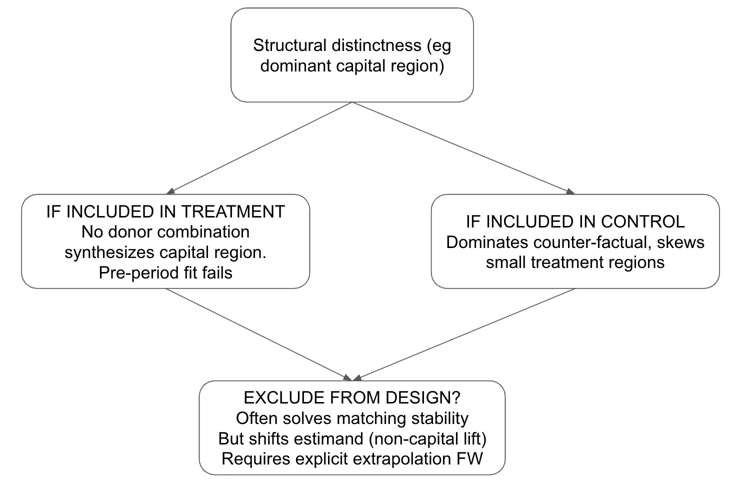
Because of this distinctness, standard matching models fail:

1. If the capital is in Treatment: no weighted combination of rural or secondary-city donor regions can synthesize its behavior. The pre-period counterfactual fit will fail validation.
2. If the capital is in Control: its sheer size and unique trend will single-handedly dominate the counterfactual for much smaller treatment regions, distorting results.

A potential solution (and its critical catch): exclude structurally distinct geos

After running dozens of iterations, experimentation teams often find that excluding the capital city or dominant hub entirely is the only way to build a stable design. Excluding a capital city can be scientifically valid, but it alters your estimand (what your experiment is actually measuring):

• You are no longer measuring national lift; you are measuring non-capital region lift.
• Extrapolating non-capital lift back to a national total becomes a separate, explicit step that requires clear business assumptions and reasoning.
• Rigor rule: capital exclusions must be pre-specified in the experiment plan, not executed post-hoc to make an unsuccessful test pass validation.

In other words, excluding the dominant hub can “save” the design analytically, but it has potentially serious implications downstream — you should carefully consider the trade-offs.

C. International cross-border contamination

In small European countries, borders are close. Mobility and ad delivery don’t stop at national frontiers:

• Cross-border workers: thousands of daily commuters cross international borders (e.g. Sweden to Denmark across the Øresund Bridge, France to Luxembourg, or Belgium to the Netherlands).
• Multi-country media spills: search, social, and programmatic campaigns frequently spill across borders in shared language blocks (e.g. the DACH region of Germany / Austria / Switzerland, or the Nordics). An ad campaign run in western Austria may inadvertently leak into southern Germany or eastern Switzerland, corrupting international control pools.

4. Practical checklist for experimentation managers

When designing or approving a geo-experiment in a smaller market, run through this practical checklist before launching:

Step	Action item	Rule of thumb / benchmark
1. Boundary selection	Use Functional Urban Areas (FUAs) or travel-to-work zones instead of postal codes.	Consult national statistics offices for commuting origin-destination matrices.
2. Mobility audit	Measure cross-region commuting shares between treatment and control candidate groups.	Under 5% share: safe to proceed. 5–10%: moderate attenuation risk — document bias direction. Over 10%: reject the partition.
3. Border buffers	Drop a geographical ring around treatment borders to absorb edge leakage.	Apply a 10–30 km buffer zone (exclude from both test and control analysis).
4. Dominant-hub check	Identify structurally distinct cities (capitals, major ports).	If a single city cannot be synthesized by donor candidate regions, pre-specify its exclusion and redefine your target estimand.
5. Instrument check	Verify that geographic region diameter is significantly larger than measurement-instrument error.	Region diameter should be at least 3–5× the expected IP drift (e.g. over 100 km for online tracking).

Summary

Geo-experimentation in smaller countries is not just a statistical optimization exercise — it is a physical identification and measurement challenge. Automated algorithms that prioritize historical pre-period fit will happily lead you into severe contamination traps if left unchecked.

By moving away from arbitrary administrative boundaries, respecting functional human mobility, and making conscious decisions about structural outliers like capital cities, you can design rigorous geo-experiments that deliver true causal insights — even in the smallest markets.